CANADIAN REAL ESTATE PRICES

IMAGE obtained from: https://lovepik.com/image-401202582/real-estate-investment.html

---

PART 1: ML & Canadian Real Estate Prices: Predicting Housing Prices Per Province with Supervised Linear Regression

---

OVERVIEW:

The motivation for this project is to ultimately integrate all of the knowledge obtained from BCS and pertain it to real life situations. This was achieved by utilizing statistics, data pre-processing and Machine Learning (ML) procedures to create relevent and predictive models regarding this topic. The final model will be presented utilizing vizualizations for ease of conveying the aforementioned data. A collaborative effort is being initiated to consider the topic of housing price indices betwee 2015-2019 with regards to population, income, crime rate, education availability and greenhouse gases across Canada, as this is a pertinent and essential topic among people in this day and age!

Primary Questions:

1. In which Province(s) can a potential buyer afford to purchase their home, based on their budget?

2. How do geographic features effect home prices in different provinces?

3. What is the projected 2020 home prices per Province, given the data gathered for this study?

Additional Questions:

• How does crime rates effect provincial population/housing prices?

• How does secondary school availability effect population/house prices?

• How does provincial greenhouse gas effect population/house prices?

We chose these Questions because:

• affordability concerns for first-time buyers/younger adults

• population alterations and migration trends across Canada

• make educated decisions regarding this big purchase, based on important features/popular current topics?

---

RESULTS:

1) PRESENTATION:

• LINK TO PRESENTATION: https://docs.google.com/presentation/d/1u-Dq1I57YpX5nCJLc6dQAZWPwopah6UY30V5wysAfAc/edit?usp=sharing

• LINKS TO SCRIBBLEMAPS:

1. INTERACTIVE HOUSE PRICES/PROVINCE:

https://www.scribblemaps.com/create/?gclid=CjwKCAjwuYWSBhByEiwAKd_n_mWpBTjhfwRO0qDbu9-bN8FImiDovtxHWmCMPVT0wdCKbbPEdYf9tBoCOXUQAvD_BwE#/id=JCrtVfTC3R&lat=53.797534&lng=-94.67929053&z=4&t=custom_style

2. INTERACTIVE PROVINCIAL POPULATIONS:

https://www.scribblemaps.com/create/?gclid=CjwKCAjwuYWSBhByEiwAKd_n_mWpBTjhfwRO0qDbu9-bN8FImiDovtxHWmCMPVT0wdCKbbPEdYf9tBoCOXUQAvD_BwE#/id=lErWy8Ic1v&lat=56.70160853&lng=-98.30477881&z=4&t=custom_style

2) GitHub: Branches were made and maintained. README and all files were updated for each Delieverable/Segment

3) DB:

This ERD depicts the relational ties between the eight tables cleaned and created in an SQL Database in preparation for analysis. With the common denominators being year and province, etc it will be determined how crime rate, greenhouse emmisions, number of post secondary educational institutions, household income, immigration income and population all contribute to shaping the choice of where to live and the effects on housing prices per province. The eight tables are as follows:

1. avg_house_prices
2. crime_rate
3. educational_institutions
4. greenhouse
5. household_income
6. immigration_median_income
7. immigration_population
8. data_by_year_prov_totals

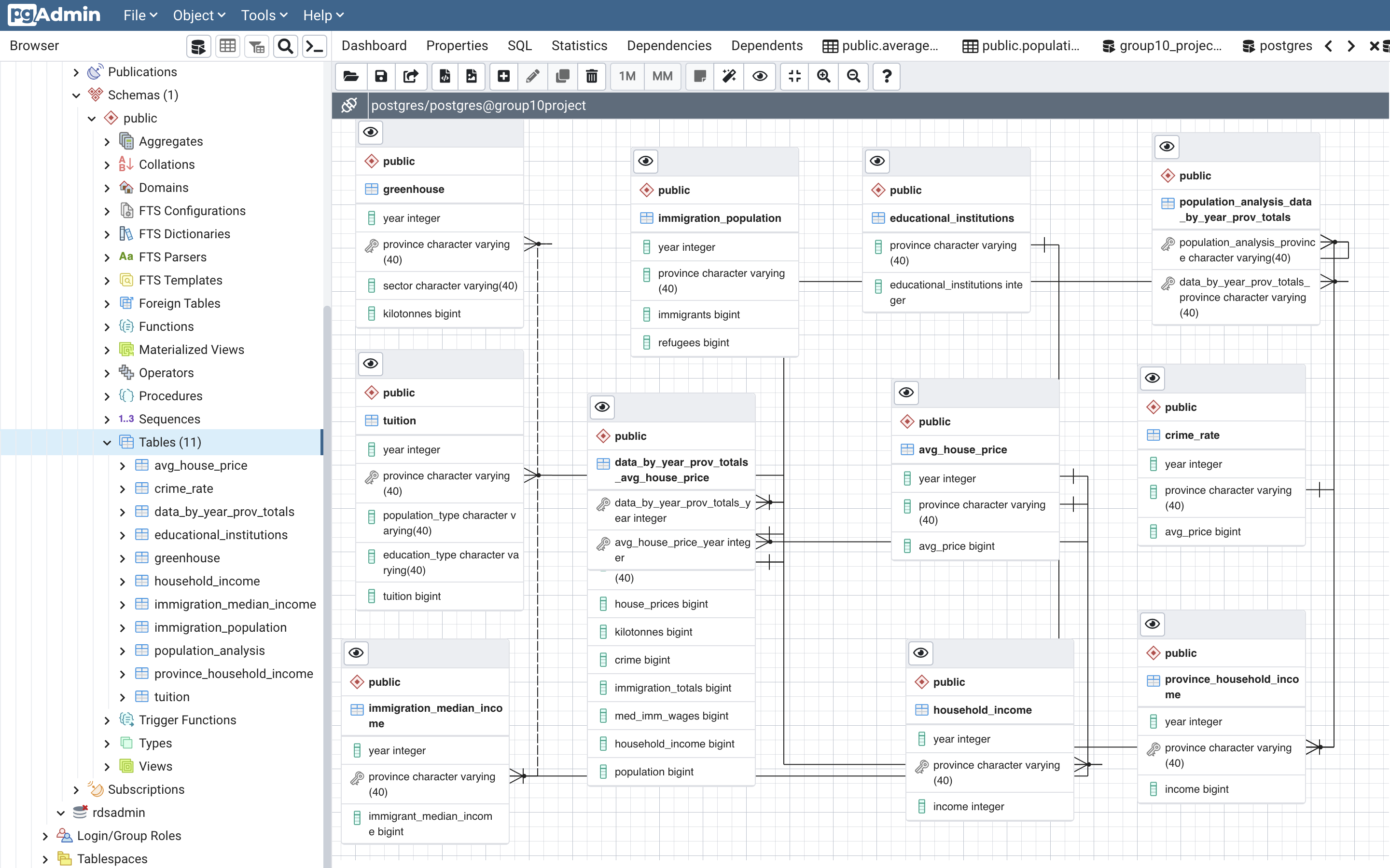
						FIGURE: ERD

Database Schema/Query

The DataBase was completed via Postgres and SQL, along with the ERD.Link: group10database.cakmngpixa6j.us-east-1.rds.amazonaws.com . A fully integrated DB connecting to the model was created, as well as 1+ joins, one connection string and an updated ERD (above) with the schema/queries below:

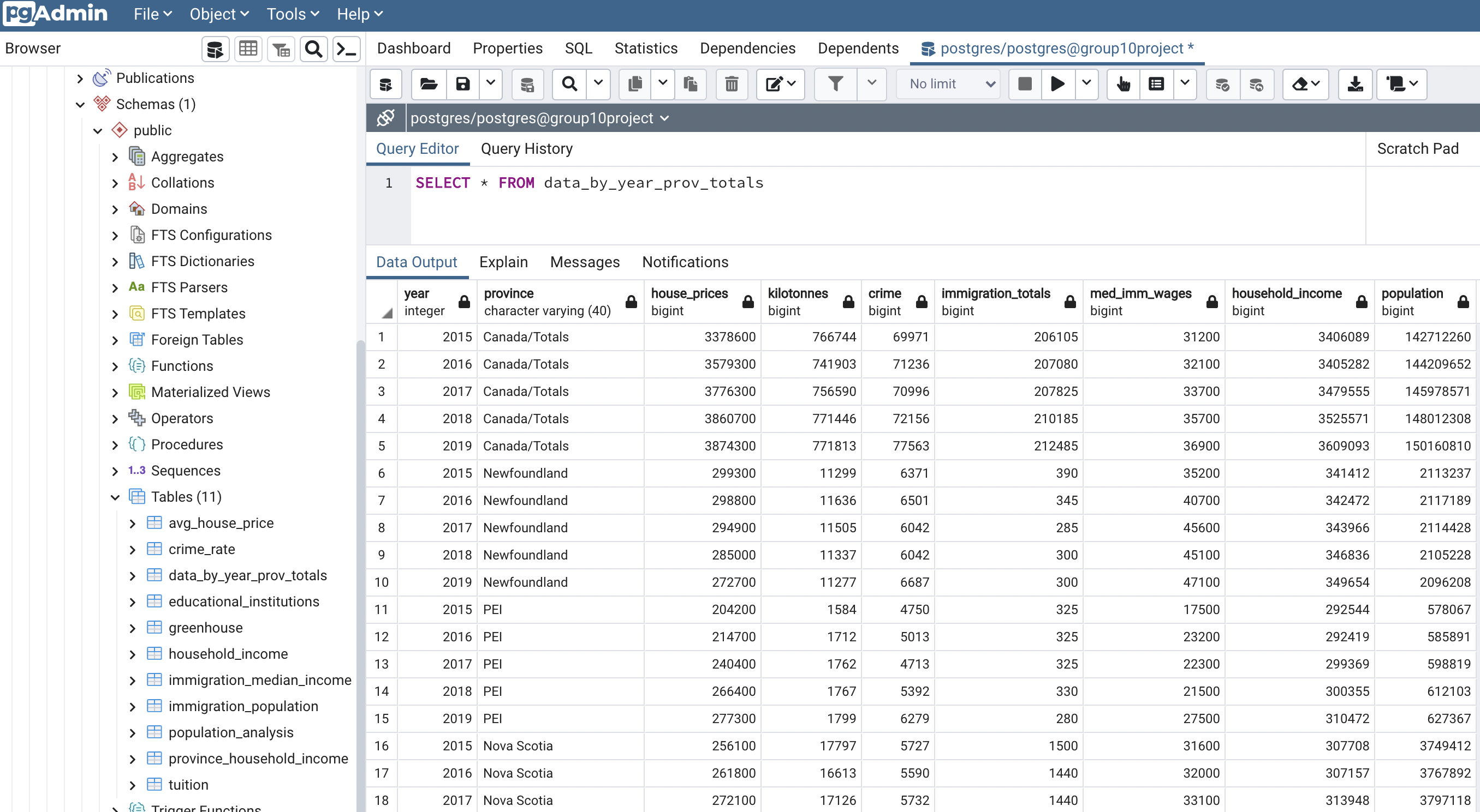
						FIGURE: SQL/Tables

CREATE TABLE household_income ( Year INT NOT NULL, Province VARCHAR(40) NOT NULL, Income INT NOT NULL );

CREATE TABLE population_analysis ( Year INT NOT NULL, Province VARCHAR(40) NOT NULL, population BIGINT NOT NULL );

CREATE TABLE avg_house_price ( Year INT NOT NULL, Province VARCHAR(40) NOT NULL, Avg_price BIGINT NOT NULL ); CREATE TABLE crime_rate ( Year INT NOT NULL, Province VARCHAR(40) NOT NULL, Avg_price BIGINT NOT NULL );

CREATE TABLE educational_institutions ( Province VARCHAR(40) NOT NULL, educational_institutions INT NOT NULL );

CREATE TABLE immigration_median_income ( Year INT NOT NULL, Province VARCHAR(40) NOT NULL, immigrant_median_income BIGINT NOT NULL );

CREATE TABLE immigration_population ( Year INT NOT NULL, Province VARCHAR(40) NOT NULL, immigrants BIGINT NOT NULL, refugees BIGINT NOT NULL );

CREATE TABLE province_household_income ( Year INT NOT NULL, Province VARCHAR(40) NOT NULL, income BIGINT NOT NULL, ); CREATE TABLE tuition ( Year INT NOT NULL, Province VARCHAR(40) NOT NULL, Population_type VARCHAR(40) NOT NULL, Education_type VARCHAR(40) NOT NULL, Tuition BIGINT NOT NULL );

CREATE TABLE greenhouse ( Year INT NOT NULL, Province VARCHAR(40) NOT NULL, Sector VARCHAR(40) NOT NULL, Kilotonnes bigint NOT NULL );

CREATE TABLE household_income ( Year INT NOT NULL, Province VARCHAR(40) NOT NULL, house_procies BIGINT NOT NULL, kilotonnes BIGINT NOT NULL, crime BIGINT NOT NULL, immigration_totals BIGINT NOT NULL, med_imm_wages BIGINT NOT NULL, household_income BIGINT NOT NULL, population BIGINT NOT NULL );

CREATE TABLE household_income ( Year INT NOT NULL, Province VARCHAR(40) NOT NULL, house_procies BIGINT NOT NULL, kilotonnes BIGINT NOT NULL, crime BIGINT NOT NULL, immigration_totals BIGINT NOT NULL, med_imm_wages BIGINT NOT NULL, household_income BIGINT NOT NULL, population BIGINT NOT NULL );

CREATE TABLE data_by_year_prov_totals ( year INT NOT NULL, province VARCHAR(40) NOT NULL, house_prices BIGINT NOT NULL, kilotonnes BIGINT NOT NULL, crime BIGINT NOT NULL, immigration_totals BIGINT NOT NULL, med_imm_wages BIGINT NOT NULL, household_income BIGINT NOT NULL, population BIGINT NOT NULL, );

4) ML MODEL:

• Description of preliminary data preprocessing:

  1. Data cleaning: Remove the irrelevant observations from the collected data, including the null values and duplicated data
  2. Data integration: combime independent variable and dependent variable each year as one table (2015-2019)
  • Independent variable: kilotonnes/Greenhouse gas, crime rate, household income, provicial population, immigration population, median immigration wage
  • Dependent variable: provincial house prices
  3. Data reduction: reduce dimensionality (scale method), create dummy data for each province (into 0 or 1)
  4. Data type transfer: change string to float type

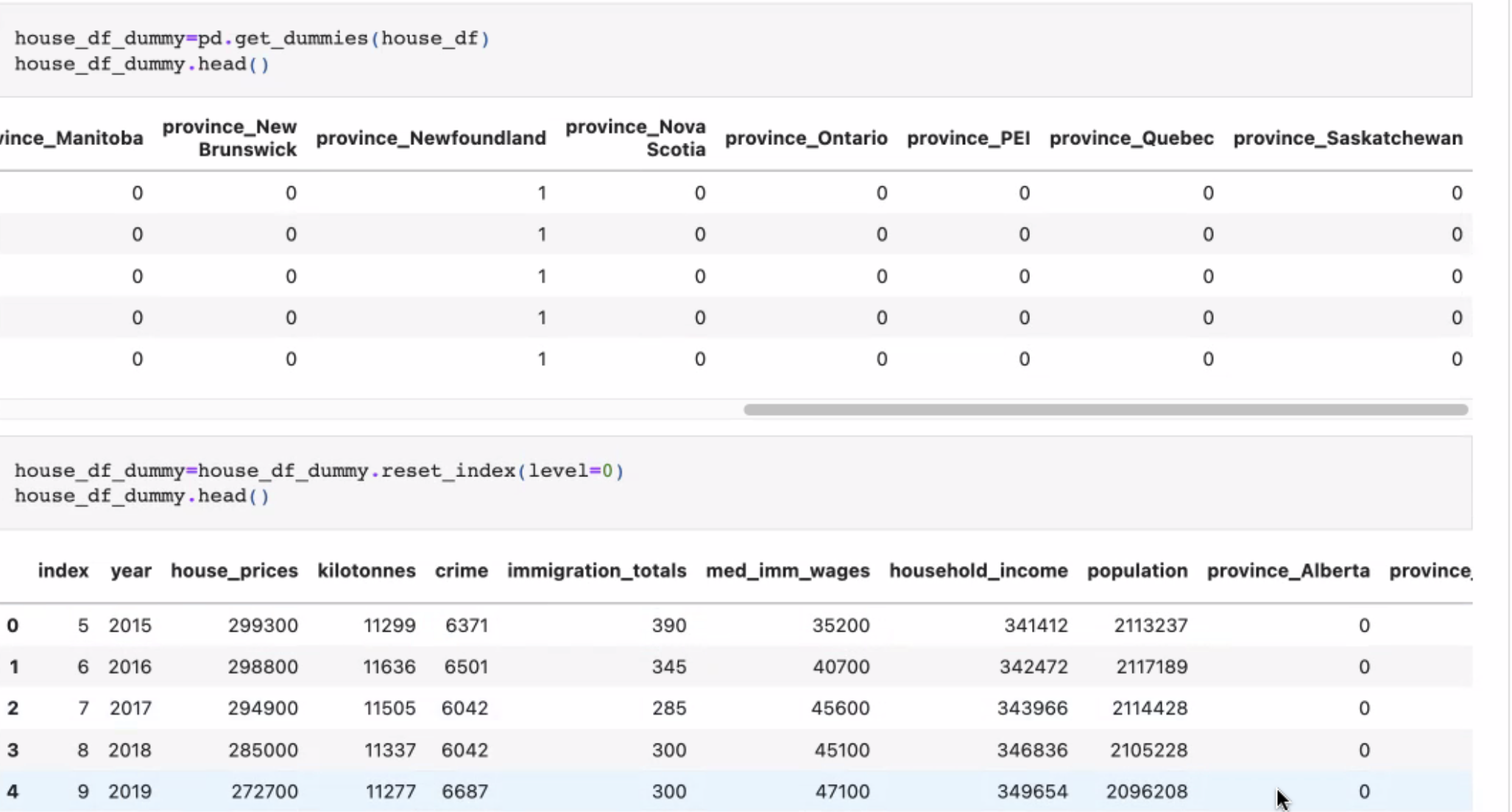
						FIGURE: Dummy Variables

• Description of preliminary feature(s) engineering and preliminary feature(s) selection, including their decision-making process:

  • Separate each province's house price from 2015 to 2019. Each line includes all the independent and dependent variables. Apply the time lag process to the previous years to forecast the future house prices

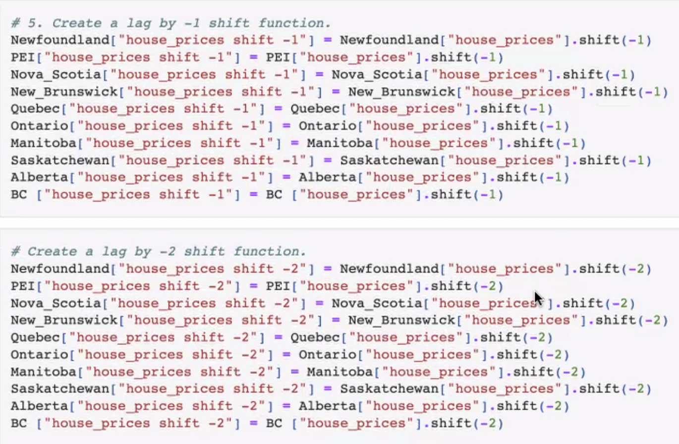
						FIGURE: Shifting -1, -2

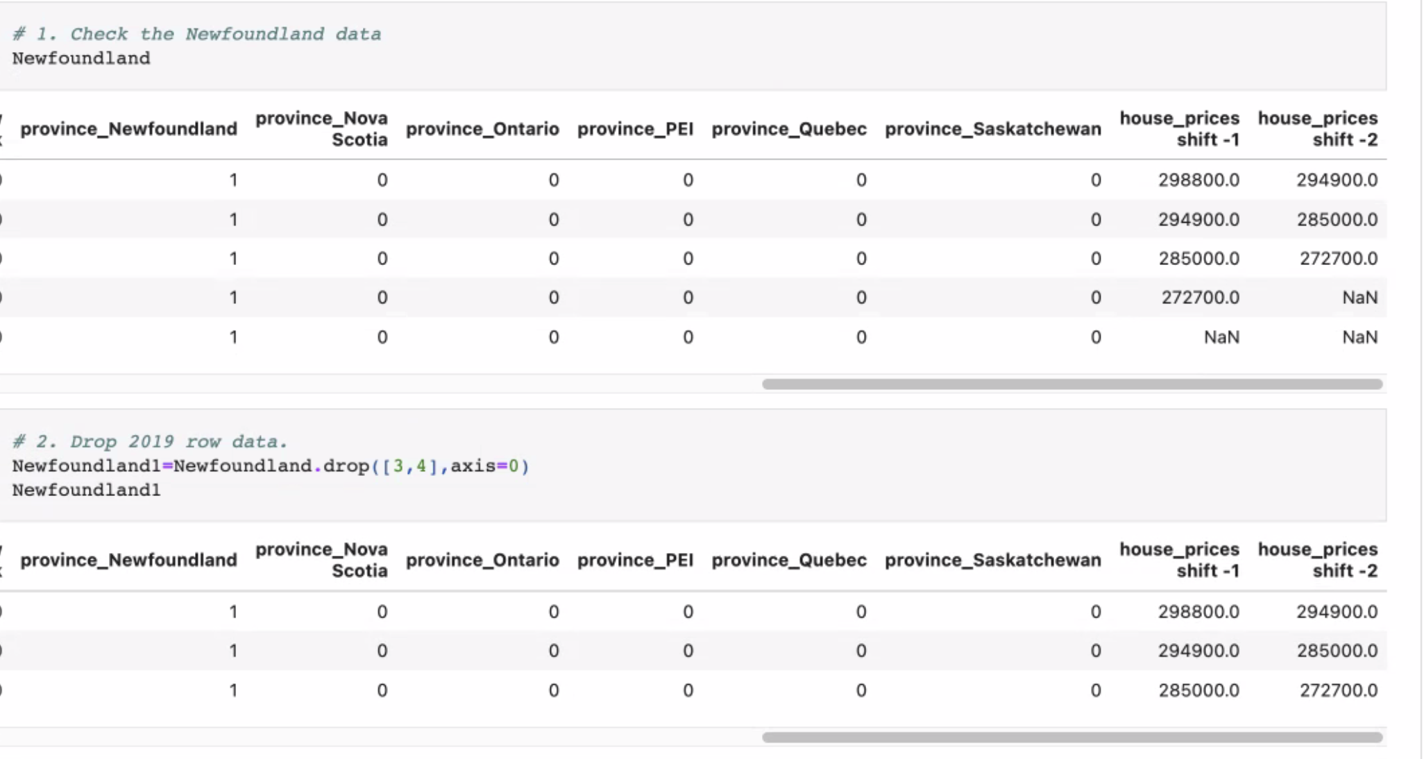
						FIGURE: Shifting

• Description of how data was split into training and testing sets:

  • 80% of dependant and independant variables are the training sets, 20% of them are test sets

• Explanation of model choice, including limitations and benefits:

  • Model: multi-variables regression

  • Description: the outcome of the analysis is continuous by each year to figure out the different variables that affect the house price. Therefore, we used the unsupervised machine learning method to analyze the future house prices. In addition, our team used three provinces to train the model based on the existing data (BC, Newfoundland, Ontario), then used the same model to predict the 2020 house prices based on the 2019 data.

  • Limitations:

    • Only can continuous numerical can be counted in data
    • We can not measure accuracy for 2020 price because we don't have the 2020 actual data to refer to/BC has low accuracy
    • The model can only show the effects of selected features and cannot analyze factors that were not selected

  • Benefits:

    • We can train and test the model to predict the future house price
    • We can used the 2018 and 2019 original values to the dataset to calculate the accurancy
    • Clearly demonstrate which factors have the greatest impact on house prices in each province

5) DASHBOARD:

The final Dashboard Presentation, including interactive/dynamic depictions for:

1) map of prices and population per province (choose prov dropdown to highlight features in 2)

2) dynamic/interactive features bubble chart for house prices (please change drop down options to 	  view different features)

3) dynamic/interactive features by budget (please chose desired budget with slider to view 		associated features)

4) Addition of Predicted Prices Bar Chart (Right)

5)Added url to github with logo (top right) on header:

link: <a href="https://lovepik.com/images/png-banking.html">Banking Png vectors by Lovepik.com</a>

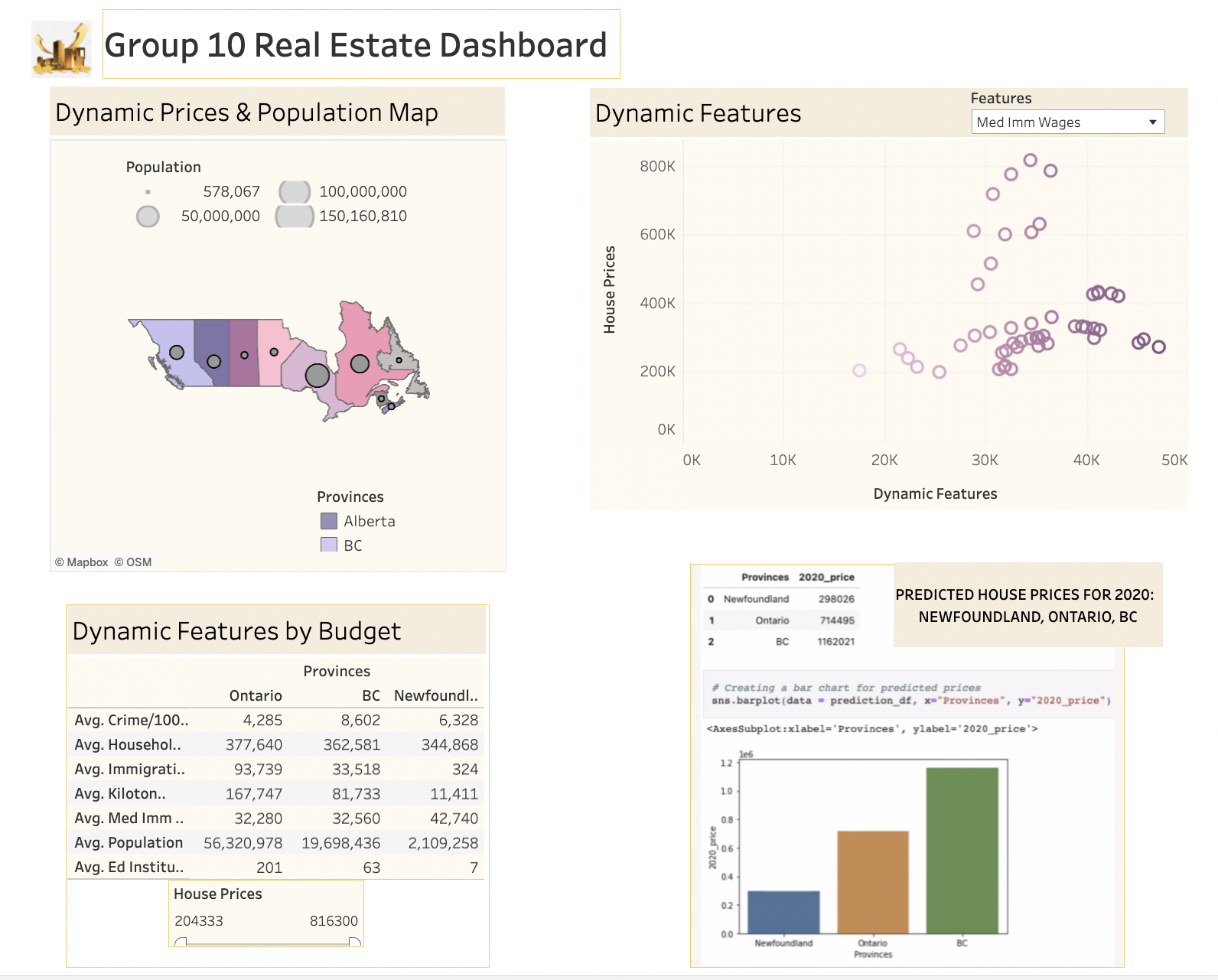
LINK: https://public.tableau.com/authoring/Group10RealEstateDashboard/Finalgroup10Dashboard#3

						FIGURE: Dashboard

CONCLUSION:

In conclusion, it can be ascertained that our model is fairly accurate, for the three Provinces that we chose: BC, Newfoundland and Ontario, with the exception of BC. As mentioned above, the limitations included the fact that we had to apply the model to each Province individually. Therefore, some recommendations would be to re-configure the model to include all of Canada, include a larger Dataset and make a more longitudinal analysis, for a more thorough study.

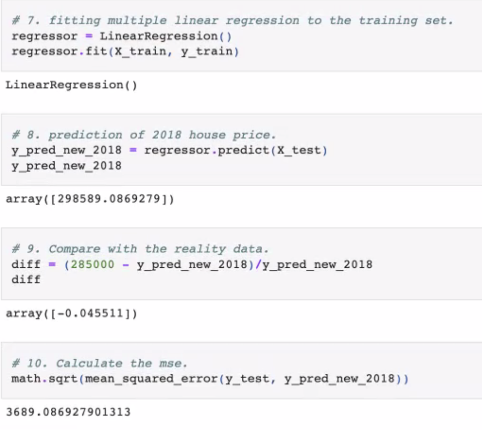
					FIGURE Predictions

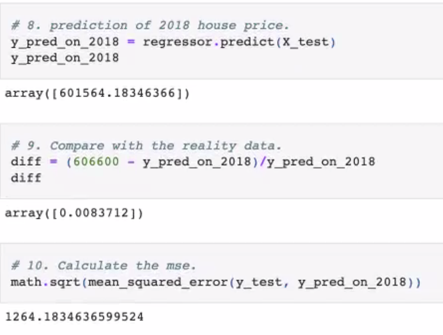
					FIGURE: Ontario Predictions

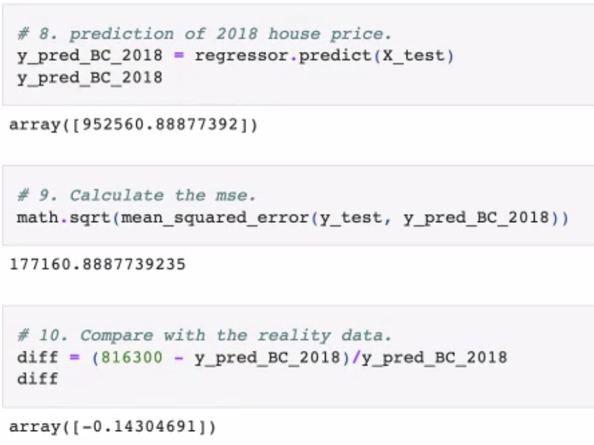
					FIGURE: BC Predictions

				FIGURE: Prediction Bar Chart for the Three Provinces

DF for prediction; our model predicts price will increase from 2019 as follows:

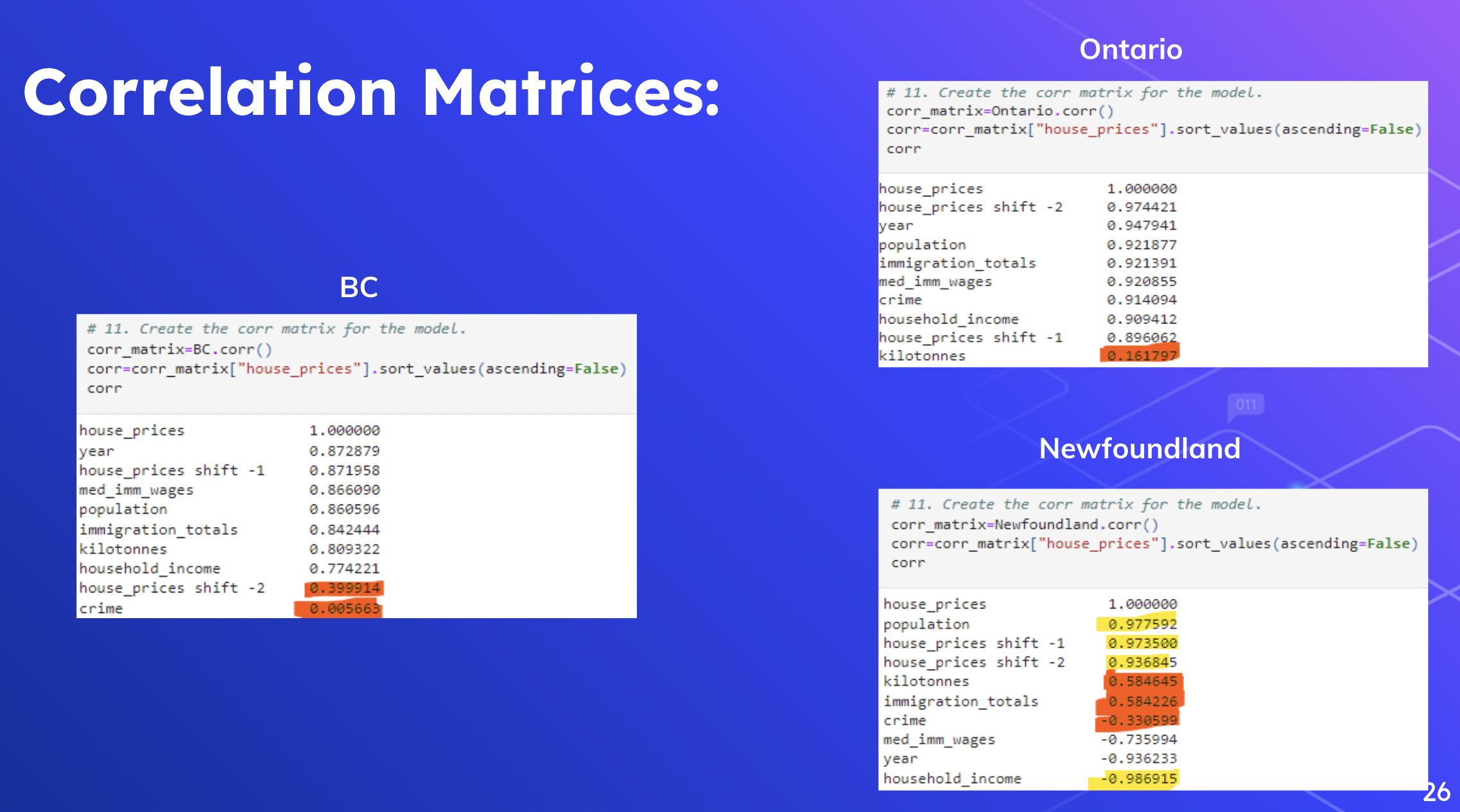
					FIGURE: Accuracy

NEWFOUNDLAND PREDICTION: 298,026; RANGE [284,465, 311,586] ACCURACY: 4.55%

ONTARIO PREDICTION: 714,495; RANGE [708,779, 720,210] ACCURACY: 0.84%

BC PREDICTION: 1,162,021; RANGE [995,851, 1,328,190] ACCURACY: 14.30%

---

PART 2: DELIVERABLES1-4:

DELIVERABLE/SEGMENT 1:

The results for Deliverable 1 encompass team collaboration via slack and with the Teaching Staff, in order to accomplish the goals. GitHub establishment requirements will be met including: initialization of an appropriate repository, addition of all branches and a README. Additionally, cleaning and pre-processing the data will be considered. A 'mockup' database will be included, as well as a potential 'mockup' ML model. Lastly, an example ERD will be included for this submission to meet all requirements. A SCRUM method of approach will be contemplated in order to attain all goals with optimal results.

1. PRESENTATION: outline with questions,mock models for DB and ML, visualizations

2. GITHUB: working code for exploratory and ML updated README, communication protocols, project outline, branches/person with 4 commits per person

3. ML MODEL: preliminary preprocessing, feature engineering and feature description with decision-making process, train and test data description, model choice with limitations and benefits

4. DB: fully integrated DB connecting to the model, 1+ joins, one connection string, updated ERD

5. DASHBOARD: blueprint, storyboard on GoogleSlides, tools and interactive slides description

DELIVERABLE/SEGMENT 2:

For this Deliverable, there will be augmentations for 5 requirements:

1. PRESENTATION: with project outline, topic and why we chose the questions, data source, description of data exploration and analysis, google slides

2. GITHUB: working code for exploratory and ML updated README, communication protocols, project outline, branches/person with 4 commits per person. Add updates, visualizations for ML, DB, presentaion, dashboard

3. ML MODEL:

• Description of preliminary data preprocessing

  • Data cleaning: Remove the irrelevant observations from collect data, including the null value and duplicate data.
  • Data intergration: combime independent variable and dependent variable each year as one table (2015-2019)
    • Independent variable: kilotonnes, crime rate, immigration population, median immigration wage, household income, provicial population.
    • Dependent variable: provincial house prices.
  • Data reduction: reduce dimensionality (scale method), create a dummy data for each province into 0 or 1.
  • Data type transfer: change string to float type.

• Description of preliminary feature engineering and preliminary feature selection, including their decision-making process

  • Separate each province's house price from 2015 to 2019. Each line includes all the independent and dependent variables. Apply the time lag process to the previous years to forecast the future house price.

• Description of how data was split into training and testing sets

  • 80% of dependant and independant variables are the training sets, 20% of them are test sets.

• Explanation of model choice, including limitations and benefits

  • Model: multi-variables regression

  • Description: the outcome of the analysis is continuous by each year to figure out the different variables that affect the house price. Therefore, we use the unsupervised machine learning method to analyze the future house price. In addition, our team used three provinces to train the model based on the existing data, then used the same model to predict the 2020 house price based on the 2019 data.

  • Limitations:

    • Only can continuous numerical can be counted in data.
    • We can not measure accuracy for 2020 price because we don't have the 2020 actual data to refer.
    • The model can only show the effects of selected features and cannot analyze factors that were not selected.

  • Benefits:

    • We can train and test the model to predict the future house price.
    • We can used the 2018 and 2019 original values to the dataset to calculate the accurancy.
    • Clearly demonstrate which factors have the greatest impact on house prices in each province.

  • Data cleaning: Remove the irrelevant observations from collect data, including the null value and duplicate data.

  • Data intergration: combime independent variable and dependent variable each year as one table (2015-2019)

    • Independent variable: provincial population, crime rate, household income, greenhouse emission, number of colleges
    • Dependent variable: house price

  • Data reduction: reduce dimensionality (reshape/scale)

  • Data type transfer: change string to float type

• Description of preliminary feature engineering and preliminary feature selection, including their decision-making process

  • Take each line as a group, for a total of 50 groups. In 2015, 5 selected characteristics were analyzed to derive each characteristic's impact (correlation) on house prices. and list the corresponding graphs (heatmaps, scatterplots, histograms)

• Description of how data was split into training and testing sets

  • Two years of data are used as the training set, and the remaining three years are used as the test set. Check whether the impact of each year's characteristics on housing prices has changed significantly or remains at a stable level.

• Explanation of model choice, including limitations and benefits

  • Model: multi-variable regression
  • Description: the outcome of the analysis is continuous by each year to figure out the different variables that affect the house price. Therefore, we use the supervised learning method. In addition, our team discovered ten provinces. Each province has 5 of the same factors that affect house prices each year, so multi-variable linear regression can help us analyze the results.
  • Limitations:
    • The model can only show the effects of selected features and cannot analyze factors that were not selected.
    • It is challenging to model nonlinear data or polynomial regression with the correlation between data features.
  • only could test a few povinces at a time
  • Benefits:
    • Visually show the impact of each element on house prices
    • Verify if these factors affect house prices to the same extent each year

4. DB: DB: fully integrated DB connecting to the model, 1+ joins, one connection string, updated ERD

5. DASHBOARD: blueprint, storyboard on GoogleSlides, tools and interactive slides description, added ML model, DB and presentation advancements

DELIVERABLE/SEGMENT 3:

1. PRESENTATION:with project outline, topic and why we chose the questions, data source, description of data exploration and analysis, google slides ADD: a more thorough description of the analysis, technologies/languages/tools and algorithms with updated slides. The slides were updated with the Revised ML Model via images with text descriptions.

2. GitHub: working code for exploratory and ML updated README, communication protocols, project outline, branches/person with 4 commits per person ADD: most of the code for ML, updated README with images/updated links, 4 commits per person. Github was updated and organized with the ML model and Data revisions, including screenshots.

3. ML model: preliminary preprocessing, feature engineering and feature description with decision-making process, train and test data description, model choice with limitations and benefits ADD: explanation in changes of model choice from last deliverable/segment, describe training/additional training, completion and description of accuracy score

REVISION TO INITIAL ML MODEL

1. In the first step, a connection to the SQL DataBase was established:

The preprocessing of the data was then initiated and the following was accomplished:

• the data was imported
• unrelated rows were dropped
• data types and null values were checked
• dummy data was obtained: .info(), .describe(), .value_counts()
• DFs were grouped by provinces
• lags were created for -1 and -2 shifts

A multi-variable Regression Model was created and Trained for 3 provinces via:

• NewFoundland data was checked
• 2019 row was dropped
• IV/DV were created
• Features (X) were separated from Target (y)
• the data was split into Training and Testing
• a Scaler instance was created and fitted
• multi linear regression was fit to the Training set
• Predictions for 2018 House Prices were established
• a Comparison was made to the 'Reality' Data
• then MSE/Correlation Matrix were created
• This process was repeated for Ontario and British Columbia

This step included the predictions for future house prices. DF's for different Provinces were utilized and lags were created for 1, 2 and 3 shifts.

4. DB: fully integrated DB connecting to the model, 1+ joins, one connection string, updated ERD ADD: ensure DB is connectable and up to date

5. DASHBOARD: blueprint, storyboard on GoogleSlides, tools and interactive slides description ADD: images/data from ML model, 1+ interative element(s). Awaiting final completed ML Model to add to Dashboard for upcoming Presentation; however, revision made to original Blueprint.

6. EXTRA: Webpage (starter) file:///Users/tanyaczeban/Desktop/webpage/index.html ?

DELIVERABLE/SEGMENT 4:

1. PRESENTATION: with project outline, topic and why we chose the questions, data source, description of data exploration and analysis, google slides ADD: a more thorough description of the analysis, technologies/languages/tools and algorithms with updated slides/images. Live presentation: all present, realtime dashboard interactivity, within time limits (7 minutes present, 5 minutes questions), speaker notes flashcards or video of presentation rehearsal

2. GITHUB: Augment readme model; production-ready code for exploratory and ML updated README, communication protocols, project outline, branches/person with 4 commits per person ADD: updated README with images/updated links, 4 commits per person, Requirements.txt file, link to dashboard and Google Slides, 16 commits in total for each team member, clean code/PEP 8

3. ML MODEL: preliminary preprocessing, feature engineering and feature description with decision-making process, train and test data description, model choice with limitations and benefits. ADD: explanation in changes of model choice from last deliverable/segment, describe training/additional training, completion and description of confusion matrix with final accuracy score

• Model Choice: multi regression, changes to shfit 1, -1, shift 2, -2, shift 3, -3

• ML model limitations: have to do for each province, could not complete R2 due to UndefinedMetricWarning/only 1 feature requiring multiple shifts

• ML Model Benefits: increase number of shifts increases accuracy

4. DB: fully integrated DB connecting to the model, 1+ joins, one connection string, updated ERD. ADD: ensure DB is connectable and up to date, holds statistic data, DB interfaces, includes 2 tables, includes 1+ join, 1 connection string (SQLAlchemy)

5. DASHBOARD: blueprint, storyboard on GoogleSlides, tools and interactive slides description. ADD: logical and easy to read, images/data from ML model, 1+ interative element(s), images or report from ML, published or screenshot.

6. EXTRA: Webpage (starter) file:///Users/tanyaczeban/Desktop/webpage/index.html ?

---

SELF_ASSESSMENT/SUMMARY:

SELF ASSESSMENT: Includes a cohesive written analysis describing:

• role played/contribution
• how contributed to other roles via discussions, peer reviews, etc.
• greatest personal challenge and how overcame it

TEAM ASSESSMENT:Includes a cohesive written analysis describing:

• teamwork
• communication protocol, challenges, resolutions and what would differently in future
• strengths as a team with tips and tricks for future cohorts

SUMMARY OF PROJECT: A 3-4 sentence summary of project (for profile, interview, etc) addressing:

• topic addressed
• machine module
• results of analysis

---

Vizualizations

Tableau, Scribblemaps, Google Slides, Python/Vsc, Pandas

https://public.tableau.com/authoring/Group10RealEstateDashboard/Finalgroup10Dashboard#3

---

Data Sources

Datasets were predominantly obtained from statscan, as well as other information sources, via a team collaborative effort. Please refer to the updated Dataset list below:

• Residential property price index, quarterly https://www150.statcan.gc.ca/t1/tbl1/en/tv.action?pid=1810016901

• Components of population change by census metropolitan area and census agglomeration, 2016 boundaries https://www150.statcan.gc.ca/t1/tbl1/en/tv.action?pid=1710013601

• Total family income and characteristics of residential property owners by family type https://www150.statcan.gc.ca/t1/tbl1/en/tv.action?pid=4610005101

• Analytical house prices indicators （country) https://stats.oecd.org/Index.aspx?DataSetCode=HOUSE_PRICES#

• Income of Immigrant tax-filers, by immigrant admission category and tax year, for Canada and provinces, 2019 constant dollars https://www150.statcan.gc.ca/t1/tbl1/en/tv.action?pid=4310002601

• Average house prices in Canada from 2014 to 2020 with a forecast up to 2022 with, by province https://www.statista.com/statistics/587661/average-house-prices-canada-by-province/

• National Price Map https://www.crea.ca/housing-market-stats/national-price-map/

• Incident-based crime statistics, by detailed violations, Canada, provinces, territories and Census Metropolitan Areas https://www150.statcan.gc.ca/t1/tbl1/en/tv.action?pid=3510017701&pickMembers%5B0%5D=1.2&pickMembers%5B1%5D=2.1&cubeTimeFrame.startYear=2015&cubeTimeFrame.endYear=2019&referencePeriods=20150101%2C20190101

• Number of Provincial Educational Institutions https://www.cicic.ca/869/RepertoireEtablissements.aspx?sortcode=2.25.26.26.27.28&p=1%2c2%2c3%2c4%2c5%2c6%2c7%2c13%2c8%2c9%2c10%2c11%2c12&t=1%2c2

• Physical flow account for greenhouse gas emissions, Frequency: Annual, Table: 38-10-0097-01 (formerly CANSIM 153-0114) Release date: 2021-12-13, Geography: Canada, Province or territory: https://www150.statcan.gc.ca/t1/tbl1/en/tv.action?pid=3810009701

• https://www.nbc.ca/content/dam/bnc/en/rates-and-analysis/economic-analysis/housing-affordability.pdf

---

Participant Names and roles

• David Baek - Database

• Siddhant Arora - Machine learning model

• Zhiyi Chen - Machine learning model

• Dylan Ruff - Database

• Tanya Czeban - Github maintain, dashboard, google slides, webpage.